
Hi everybody,
I decided to play around with LLaMa3 based architecture, implement it in pytorch and gradually optimise it for training speed to see how far I can get (and with how much effort... The Sky is the limit after all.) Spoiler alert, I can easily reach 9X faster training!
Background information:
Why LLaMa3?
It's not a MoE, relatively simple architecture upon which we can iterate. The goal is to focus on a mature well established architecture and apply common speed up techniques, more so than cutting edge transformer variants.
Did you implement it yourself?
No, I adapted the code from this blog post.
I changed the RoPE implementation to one from the official (but now deprecated) LLaMa3 repo, and I replaced the RMSNorm implementation with the one that is provided in the pytorch module. I also modified the default model definition to something bigger, compared to what is used in the blog post, and also used the AdamW optimizer with a CosineLR scheduler, because any real NN training should use a LR scheduler on top of an optimiser.
Model definition
As I wanted to keep the model size manageable for training on a single GPU, I used a relatively small model (16 layers, 16 heads, 16 kv-heads, 1024 model dim, 256 max seq len, 1000 Epochs). In this setup, an output layer with the full LLaMa3 vocab (100k+ tokens) will be the single most expensive operation in the model and will kind'a overshadow performance improvements we can do elsewhere. Instead, I'll use a char based vocab of 68 tokens, which will better mimic a real world scenario. This resulting model has 103M parameters.
Optimisations
I'm mostly looking at increasing training speed, without affecting much the training loss. I will start with methods that don't change the model and gradually move to methods that change the model. After all, we care about getting a comparable validation loss achieved in less real time. A comprehensive approach will optimise both the code AND the model architecture.
Training set
I grabbed a training set tittled tiny_shakespeare from the repository of the author of the otiginal blog post. 80% of the 40k lines are used as a train set, the other 20% are split equally between validation and test set.
Baseline run
The baseline run produces the following scores:
...
Epoch 970 | val loss 2.222 | Time 1.173
Epoch 980 | val loss 2.171 | Time 1.174
Epoch 990 | val loss 2.213 | Time 1.173
validation loss: 2.2126235485076906
We are aiming to reduce the Time it takes to complete 10 epochs, whilst maintaining comparable loss. The mini_batch size is 10 and I'll avoid touching it for now, because that's a more trivially tunable parameter, and it seems it's big enough for my 3090.
The code for the baseline run can be found here.
Non-Model Optimisation journey
Now, let's get started optimising. In this section we will talk only about optimisation techniques that DO NOT change the model
Floating Point precision
The first thing to do is to change the default type from float32 to bfloat16, as my GPU (and any modern GPU) should support that. bf16 is half the bytes of fp32, but unlike fp16, it maintains the same dynamic range, at cost of less precision after the decimal point. This property of bf16 is very useful, because it avoids numerical issues with very large numbers, and is trivially convertible to/from fp32 as they have the same number of exponent bits.
While in very big neural networks, numerical issues may arise in gradient summation, as shown here but for our comparatively tiny case, this is a free win we can take:
torch.set_default_dtype(torch.bfloat16)
...
Epoch 970 | val loss 2.221 | Time 0.510
Epoch 980 | val loss 2.214 | Time 0.511
Epoch 990 | val loss 2.213 | Time 0.511
validation loss: 2.2131337881088258
And, just like that 2x speedup, basically for free.
Fused/Optimised operations
One of the big performance boosts we can get is from fusing operations. Fusing essentially means chaining operations together, so that we avoid writing intermediate results to memory and then reading them back. A very basic example would be if we have ReLU(X*W), instead of completing the multiplication first, writing it to memory, and then reading it again, we insert the ReLU operator inside the GEMM routine.
Writing those is complicated, and GPU architecture dependent. Luckily of us some libraries that implement those exist, such as Facebook's xformers. Note that not all optimised operators are strictly speaking "Fused". Sometimes, it's a more memory efficient implementation, sometimes the algorithm is significantly modified in a mathematically equivalent way, such as in flash attention.
The point is that those are complex custom implementations of operators that differ significantly from the pytorch implementation, come with some caveats and limitations, but usually result in significant performance improvements.
Fused SwiGLU
Optimised SwiGLU op is available in xformers and we can make use of it. We just replace our FeedForward layer implementation:
class FeedForward(nn.Module):
  def __init__(self, dim:int, hidden_dim:int, multiple_of:int, ffn_dim_multiplier: Optional[float]):
    super().__init__()
    # Models embedding dimension
    self.dim = dim

    # We must use the hidden dimensions calculation shared by Meta which is the ideal one for this model
    # Hidden dimension are calculated such that it is a multiple of 256.
    hidden_dim = int(2 * hidden_dim/3)
    if ffn_dim_multiplier is not None:
      hidden_dim = int(ffn_dim_multiplier * hidden_dim)
    hidden_dim = multiple_of * ((hidden_dim + multiple_of - 1) // multiple_of)

    # define hiddne layers weights
    self.w1 = nn.Linear(self.dim, hidden_dim, bias=False, device=device)
    self.w2 = nn.Linear(hidden_dim, self.dim, bias=False, device=device)
    self.w3 = nn.Linear(self.dim, hidden_dim, bias=False, device=device)

  def forward(self, x):
    # Shape: [bsz,seq_len,dim]
    return self.w2(F.silu(self.w1(x)) * self.w3(x))
...
self.feedforward = FeedForward(args.dim, 4 * args.dim, args.multiple_of, args.ffn_dim_multiplier)
With
from xformers.ops.swiglu_op import SwiGLU
self.feedforward = SwiGLU(1024, 2816, bias = False) # This results in the same number of parameters as the FeedForward implementation
...
Epoch 970 | val loss 2.248 | Time 0.491
Epoch 980 | val loss 2.212 | Time 0.490
Epoch 990 | val loss 2.186 | Time 0.491
validation loss: 2.1855790853500365
And we get another 5% performance boost. Note that I've hardcoded the input and output dimensions in the SwiGLU op because they are calculated slightly differently from the initial FeedForward implementation.
Fused attention.
Everybody knows that the attention mechanism is extremely expensive due to its n**2 computational complexity which scales with sequence length. It is usually the biggest blocker when it comes to computational efficiency and long context.
We are going to replace this code:
 # To compute attention, we'll need to perform a transpose operation to reshape all queries, keys and values bring heads at dim 1 and seq at dim 2
xq = xq.transpose(1,2)                  #xq[bsz,n_heads,seq_len,head_dim]
keys = keys.transpose(1,2)              #keys[bsz,n_heads,seq_len,head_dim]
values = values.transpose(1,2)          #values[bsz,n_heads,seq_len,head_dim]

# Computing attention score
scores = torch.matmul(xq, keys.transpose(2,3)).to(self.args.device)/math.sqrt(self.head_dim)
if mask is not None:
    scores = scores + mask

# Apply softmax to the attention score
scores = F.softmax(scores.float(), dim=-1).type_as(xq)
# Matrix multiplication of attention score with the values
output = torch.matmul(scores, values).to(self.args.device)
with
# To compute attention, we'll need to perform a transpose operation to reshape all queries, keys and values bring heads at dim 1 and seq at dim 2
xq = xq.transpose(1,2)                  #xq[bsz,n_heads,seq_len,head_dim]
keys = keys.transpose(1,2)              #keys[bsz,n_heads,seq_len,head_dim]
values = values.transpose(1,2)          #values[bsz,n_heads,seq_len,head_dim]
output = F.scaled_dot_product_attention(xq,keys,values, mask)
...
Epoch 970 | val loss 2.186 | Time 0.402
Epoch 980 | val loss 2.223 | Time 0.401
Epoch 990 | val loss 2.249 | Time 0.402
validation loss: 2.2491623640060423
Some slight numerical differences are to be anticipated, so the resulting convergence is not exactly the same, but it is comparable, and we shaved off nearly 20% of the runtime! On top of that, this attention uses less memory which is important in many real world scenarios where we are always maxing out the available memory.
Note that there are many efficient attention implementations. Please consult pytorch's extensive documentation on the subject. Unfortunately there wasn't a flash attention kernel compiled for my 3090 and I didn't bother to compile pytorch with it, so I didn't test it.
Techniques I didn't try
Optimisation is an endless journey and very model and hardware dependent. There are a number of things to try that are not applicable to my scenario/hardware:
- Mixed precision training. Going down to fp8 and even fp4, with gradients in bf16/fp32 is commonly done when training frontier models. nvidia showcased we can train in FP4 without loss in accuracy, but accelerated fp4 hardware is available on GPUs of later generation than mine.
- Different types of model sharding when doing multidevice training were not looked at, as I only have one GPU. When working with big models, especially Mixture of Experts, we have a number of different types of parallelism: Data Parallelism, Tensor Parallelism, Pipeline Parallelism, Expert Parallelism, etc... Making good use of those will minimise the gaps in our pipelines and the idling of our GPUs.
- For inference, there's tons of quantisation methods out there, but I will leave them as outside the scope of this tutorial.
Results of pure code optimisation
We have roughly achieved 3X faster training by using more efficient implementation without writing any custom kernels. We can always do more, we can fuse more operators, we can use search for better hyperparameters... If we do want to optimise further the best thing to do is to PROFILE.
Profiling
When spending effort to improve performance, we want to start from the biggest offenders first and work down the line. How do we find those? Through profiling. Profiling in pytorch is easy, just refer to the documentation:
from torch.profiler import profile, ProfilerActivity, record_function
...
with profile(activities=[ProfilerActivity.CUDA], record_shapes=True) as prof:
  with record_function("model_inference"):
    train_results = train(model, optimizer, ModelArgs)
prof_key_average = prof.key_averages()
with open('/tmp/tst', 'w') as myout:
    myout.write(prof_key_average.table(sort_by="cuda_time_total", row_limit=20, max_name_column_width=1600))
Then open the resulting file with really long lines and inspect the result. For best view, download the file open in your favourite text editor and disable word wrap.
The top offender is Fused GEMM+Swiglu kernel with 1/4th of the total runtime, and attention is coming in only 4th-5th place. If you struggle with decoding the long function names, google/AI is your friend.
Model Optimisation Journey
Work smarter, not harder. If we can make a model that learns just as fast (or even faster!) in terms of epochs, but is smaller, we can get some extra wins in terms of wall clock time!
Grouped Query Attention
One common mechanism to reduce the cost of attention is to reduce the number of KV heads to a smaller amount. Maybe for every two Queries you only need a single KV pair? The intuition behind it is that the information from KV heads is largely redundant and not all of them are necessary:
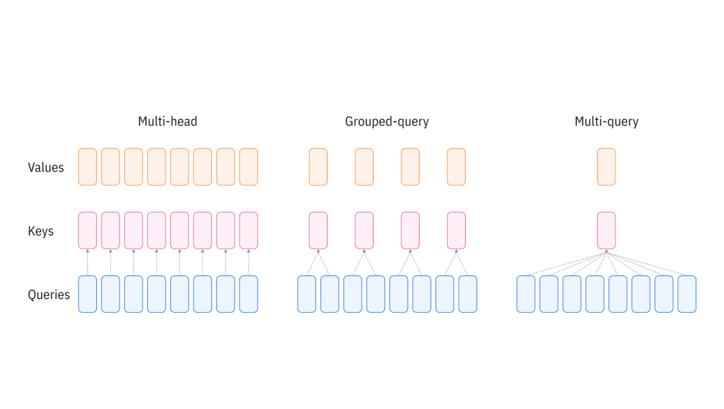
If you are interested in more information, please check out the MQA and the GQA papers.
Modifying our code is trivial, because the pytorch attention implementation supports GQA with the extra argument enable_gqa=True. Let's just halve the KV heads and give it a go:
...
n_heads: int = 16            # number of heads for queries embedding
n_kv_heads: int = 8         # number of heads for keys and values embedding
...
output = F.scaled_dot_product_attention(xq,keys,values, mask, enable_gqa=True)
Epoch 970 | val loss 2.226 | Time 0.519
Epoch 980 | val loss 2.215 | Time 0.548
Epoch 990 | val loss 2.262 | Time 0.520
validation loss: 2.261601686477661
Well, shit, we got slower!? Well, turns out GQA is supported only in flash_attention, which is pytorch didn't compile for my architecture, so I fallback on the basic pytorch implementation, which is slow.
Fear not, for if the attention implementation doesn't support it, we can always use a repeat/reshape function that repeats and concatenates grouped KV heads onto themselves, so that the attention does the computation with full heads:
# If the number of keys/values heads is fewer than query heads, this function expands the key/values embeddings with the required number of repetition
def repeat_kv(x:torch.Tensor, n_rep: int)-> torch.Tensor:
  bsz, seq_len, n_kv_heads, head_dim = x.shape
  if n_rep == 1:
    return x
  return (
      x[:,:,:,None,:]
      .expand(bsz,seq_len,n_kv_heads,n_rep, head_dim)
      .reshape(bsz,seq_len,n_kv_heads * n_rep, head_dim)
  )
...
Epoch 970 | val loss 2.242 | Time 0.385
Epoch 980 | val loss 2.213 | Time 0.388
Epoch 990 | val loss 2.206 | Time 0.386
validation loss: 2.2057207822799683
Now the model is smaller, down to 94.5M parameters, and we are faster, with another 5% performance improvement. It's important to note that while GQA is faster than pure MHA, it is less expressive and reducing the number of KV heads too much will lead to obvious performance issues. GQA is especially beneficial during decoding as it will drastically reduce the memory requirements for the KV cache.
The code for the optimised run can be found here.
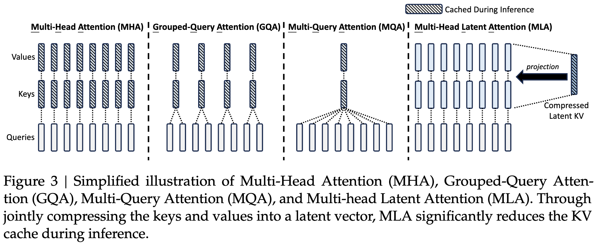
Deepseek latent attention
Deepseek introduces latent attention, meaning the KV matrices are downprojected to low dimensional space and uprojected to the high dimensional space during computation. In practise this means that the KV cache is tiny, less than 10% of the size compared to full KV matrices, and the model has less parameters: just 82.4M.
I changed the attention of my model to deepseek style one, adapted from this blog post. The resulting code can be found here.
Epoch 970 | val loss 1.415 | Time 0.377
Epoch 980 | val loss 1.418 | Time 0.376
Epoch 990 | val loss 1.413 | Time 0.377
validation loss: 1.4130668997764588
Not only is the resulting model a few percent faster, but it converges much much faster and to a better point.
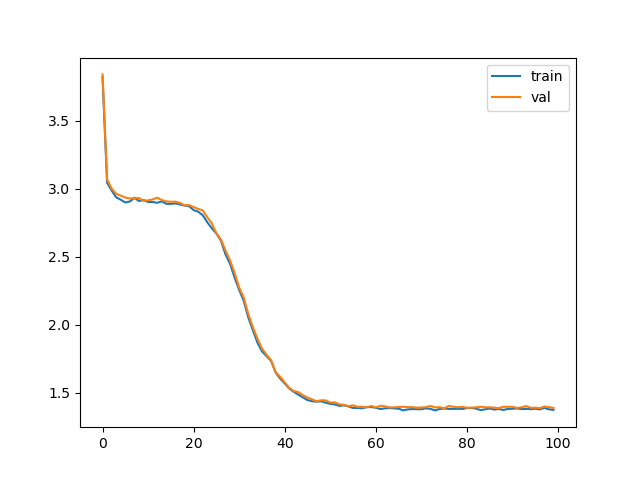
My intuition about why convergence is faster here is that the simpler deepseek attention with less parameters is actually easier to learn and our very simple dataset does not require the expressiveness of full attention. It is remarkable what huge difference the architecture makes, we are nearly halving the loss average.
If we consider the overall speedup in terms of real time to reach similar perplexity, it is easily 3X compared to the best optimised model. If we compare to the baseline implementation, we are reaching 8-9X speedup!
Conclusion
Good optimisation is always achieved through both code and model improvements. Through code improvements alone, we can reach about 2.5X speedup, but through modelling improvements we can reach 8-9X faster convergence.
We should also look at inference performance, but this blog post is getting kind'a long so I will stop here.